Transient Heat Flow Example
The files related to this example are contained in TransientHeatFlow.zip
Introduction
FEMM has the capability to perform transient heat flow analyses, given the constraint that the finite element mesh cannot change from time step to time step. The purpose of this note is to provide a concrete example of the use of the heat flow time transient functionality.
Problem Description
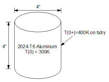
The problem domain is a 4 inch X 4 inch cylinder of 2024-T6 Aluminum. The prior to time \(t=0\), the entire cylinder is at a steady temperature of 300K. At \(t=0\), the temperature of the external boundaries is changed to 400K. The problem domain is shown as Figure 1. The goal of the problem is to model the evolution of the temperature in the cylinder over the timespan from \(t=0\) to \(t=20\) seconds.

Figure 1: Example transient heat flow problem domain.
Equations
For heat flow transient problems, FEMM solves the heat equation:
\[ \large \rho c_p \frac{dT}{dt} - \nabla \cdot \left( k \nabla T \right) = q \]
The program uses an implicit Euler time discretization scheme. That is, given the solution at time \(n-1\), the equation solved by FEMM to step the solution forward one step in time to time \(n\) is:
\[ \large \rho c_p \left( \frac{T_n - T_{n-1}}{\Delta t} \right) - \nabla \cdot \left( k \nabla T_n \right) = q \]
The material properties in the equation are the volumetric heat capacity (\(\rho c_p\)) and thermal conductivity (\(k\)). The problem is driven by volumetric heat generation (\(q\)). Heat can also enter and exit the problem through boundaries, depending on the definition of the boundary conditions.
Problem Solution
First, a FEMM problem is made to model the initial condition. This problem is saved as T0.feh in TransientHeatFlow.zip. The cylinder is modeled with a 300K boundary condition applied on all external edges of the domain, then solved by pressing the "turn the crank" toolbar button. The solution file, T0.anh, serves as the initial condition for the transient problem.
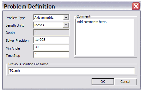
To step to the next time step, a second file, T1.feh, is then created. This file is identical to T0.feh, except that a 400K boundary condition is applied to all external boundaries. To turn the problem from a steady-state problem into a step in a transient problem, fields in the "Problem Definition" dialog (Select "Problem" off of the main menu) must be altered. Referring to Figure 2, a "previous solution file name" is first prescribed. For this step of the problem, the solution of the initial condition, T0.anh, should be specified. When a previous solution file name is specified, the "Time Step" field will be enabled. For the purposes of this example, a 1 second time step can be used.

Figure 2: Heat Flow Problem Definition Dialog.
The problem can then be evaluated, and the resulting T1.anh will be the answer for the solution stepped forward one step in time.
To model addition time steps, a file named T2.feh referring to the solution T1.anh and so on.
Scripting
Although it is possible to manually step the program through a series of solutions for different time steps, performing this task manually is somewhat tedious. It is much more convenient to create a short script in one of the FEMM-supported languages (Lua, Matlab, Octave, Scilab, or Mathematica) to automatically generate the sequence of solutions. For this example, a Lua script was created. The script below automates the actions described above, generating a sequence of 20 time steps at 1 second increments. This particular script also saves a picture of each solution as a bitmap so that a movie of the evolution of the solution over time can be created.
-- Create an initial condition answer file
-- This solution has a fixed 300K applied to
-- the boundaries of the domain.
open("T0.feh");
hi_analyze();
hi_close();
-- Load the first transient solution file.
-- The difference betweeen T0.feh and T1.feh is that
-- T1 has a different boundary condition applied to the edge
-- that will drive the temperature up to a new steady-state of 400K
open("T1.feh");
for n=1,20 do
-- Modify to the problem definition to point to the
-- solution from the previous iteration. The program will step
-- the solution forward from the previous step using an implicit
-- Euler time integration scheme.
-- For this particular case, a 1s time step has been selected.
hi_probdef("inches","axi",1.e-8,1,30,"T"..(n-1)..".anh",1);
hi_saveas("T"..n..".feh");
hi_analyze();
-- Save a screenshot of each solution so that they
-- can be strung together into a movie
hi_loadsolution();
--ho showdensityplot(legend,gscale,type,upper,lower)
ho_showdensityplot(1,0,0,400,300,0);
ho_savebitmap("T"..n..".bmp");
ho_close();
end
hi_close();
The script is run by clicking the "Open a Lua script" button on the top of the left-hand toolbars. When the script is run, it will generate solution, answer, and bitmap files for each time step.
Animation
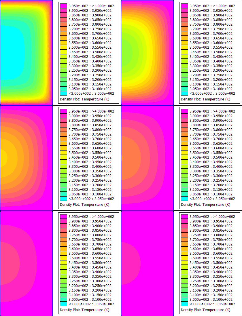
For this example, the bitmap files were converted to gif files using the convert command line program from ImageMagick. GIF Animator can be used to glue all of the gif files into one animated gif. The resulting animation is shown below as Figure 3.

Figure 3: Animated transient heat flow solution.
Conclusions
This note has presented a simple example of the use of FEMM's transient heat flow capabilities. Although this example is relatively simple, it is possible to solve more elaborate problems where the heat sources vary on a step-by-step basis, perhaps in concert with the results of an AC magnetics analysis. However, all transient heat flow solutions follow essentially the same time stepping solution process.