Random Optimization with FEMM
Issues that influence the application of optimization methods to FEMM problems include:
- Expensive Cost Function Evaluation. Each cost function evaluation requires a finite element analysis.
- Discontinuous Search Space. Because of discretization error associated with remeshing, cost functions typically don't vary smoothly or continuously vs. geometry.
Random Optimization is a powerful method for use with finite element analysis because it accommodates both of these difficult issues. With inspiration from the Wikipedia page, the variant of the algorithm considered here is:
Let \(f\): ℝn → ℝ be the fitness or cost function which must be minimized. Let \(x\) ∈ ℝn designate a position or candidate solution in the search-space. The algorithm can then be described as:
- Initialize x with a random position in the search-space.
- Until a termination criterion is met (e.g. number of iterations performed, or adequate fitness reached), repeat the following:
- Sample a new position y from the hypercube of a given radius surrounding the current position \(x\)
- If \(f(y) < f(x)\) then move to the new position by setting \( x = y \)
- Now x holds the best-found position.
- If there is no progress in \(m\) iterations, shrink each linear dimension of the hypercube by a factor of 2.
This algorithm is good with respect to expensive function evaluation because only one function evaluation is needed to generate the next potential step. It is also well-suited to the discontinuous nature of cost functions applied to finite element programs, since it jumps to new optima rather than smoothly traveling. This feature tends to reject most local minima. Constraints are also easy to accommodate--if a randomly generated candidate solution doesn't meet all applicable constraints, it is simply rejected.
Example: Minimization of a Simple Function
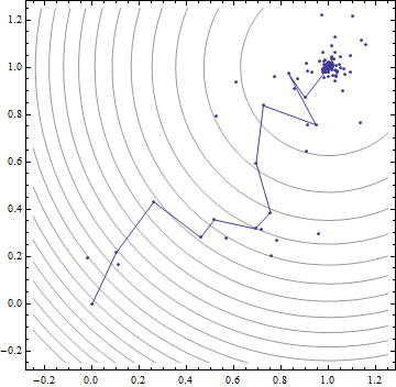
Before applying the method to a finite element problem, it is instructive to apply it to a simple problem with a known solution. Let cost function f be defined as:
\( f = (x_1 - 1)^2 + (x_2 - 1)^2 \)
In this case, \(f\) is a 2D quadratic function that is minimized at \([x_1,x_2] = [1,1]\). Although RO is an inefficient way to solve this particular optimization, it is an easily understandable and graphable problem. A Mathematica implementation of the algorithm is as follows:
R[]:=Random[]*2-1
f[X_] := (X - {1, 1}).(X - {1, 1})

d = 0.25;
m = 10;
stall = 0;
X = {0, 0};
fbest =  f[X];
For[k = 1, k < 1000, k++,
	Xnew = X + d*{R[], R[]};
	fnew = f[Xnew];
	stall++;
	If[fnew < fbest,
		fbest = fnew;
  		X = Xnew;
  		stall = 0;
  		Print[k, "  ", d, "  ", X];
  	];
 	If[stall == m,
  		stall = 0;
  		d = d/2;
  	];
 	If[d < 0.001, Break[]]
 ]
The output of the program, with the iteration number, step size, and position for each cost function-reducing move, is:
|
|
Example: Finite Element Geometry Optimization
This same method can be used to optimize the geometry of a magnetic device. This example uses a set of Matlab functions to optimize 14-magnet outrunner-type brushless DC motor of the type commonly used to propel small UAVs. For this example, the script seeks to minimize the size of the motor, given a specified bulk current density in the windings and a desired torque that should be produced at the specified current density. The script calls FEMM on candidate geometries to figure out how much torque the cross-section produced per unit length so that the required axial length of the machine can be determined. The script explores a series of candidate geometries using the same random optimization procedure as described in the simple example above.
A zip archive containing the example files is here: SPSOpt.zip
Conclusions
A "random optimization" procedure has been presented that is relatively easy to implement and works geometries analyzed by FEMM. The example motor optimization demonstrates that the procedure can be used to optimize the design of electric machine with many parameters and design constraints.
