Determination of Transformer Operating Point

David Meeker

August 10, 2006

Introduction

For time-harmonic magnetic problems in FEMM 4.0, windings with specified currents can be modeled, and the voltage drop across these windings can be computed as an analysis result. However, it is often the case that one would like to specify the voltage across a winding and compute the resulting current. The case of a transformer is even more difficult—one generally would like to specify a voltage across the primary of the transformer and the secondary load impedance and obtain the resulting operating currents in the transformer. The following note describes an example Octave script that uses a series of runs to iteratively determine a simple transformer’s operating point.

Example Geometry

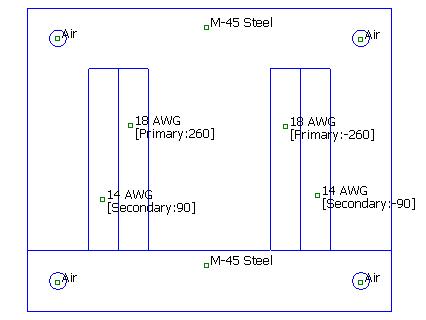
The single-phase isolation transformer considered in this note is shown in Figure 1. This particular transformer has 260 turns in the primary and 90 turns in the secondary, reducing a 120 V_rms input on the primary to approximately 40 V_rms across the secondary. The dimensions of the transformer core are .

Figure 1: Single-phase EI transformer.

Although a number of interesting effects could be considered, such as:

The effect of the small air gaps at lamination joints
Rolling direction
End turn impedance

these effect are neglected here for the purposes of simplicity of the example. However, it can be noted that the following effects are “automatically” included by the material property definitions used in the example:

Hysteresis and eddy current loss in the laminations
Proximity and skin effects in the transformer windings

Derivation of Iterative Method

Some sort of automatic iterative method for determining the operating currents is desired. With more than one current, it is nearly impossible to tune the currents by hand to obtain a particular operating point. If the problem were linear, two equations relating the applied voltages and resulting currents could be written as:

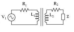
These equations correspond to the circuit diagram pictured in Figure 2:

Figure 2: Transformer circuit diagram.

Resistances R₁ and R₂ represent the internal resistance of the transformer. Inductances L₁ and L₂ represent the self-inductances of the primary and secondary windings, respectively. Mutual inductance M links the two windings. The mutual inductance is closely related to the self-inductances:

where the difference between these quantities depend on the amount of leakage inductance in the transformer. Impedance Z is the load impedance attached to the transformer.

The equations could be more succinctly written in matrix notation as:

(1)

where the transformer internal impedance matrix Z_t is defined as:

the load impedance matrix Z_l is defined as:

\[ Z_l = \left[ \begin{array}{cc} 0 & 0 \\ 0 & Z \end{array}\right] \]
the voltage vector is defined as:

and the current vector is:

We could further defined the voltage drop over just the transformer impedance to be v_t, by definition:

(2)

Equations (1) and (2) can be added together to yield:

(3)

Eq. (3) can be re-arranged as:

(4)

This development suggests an iterative method for determining the operating currents in a transformer in FEMM:

(5)

where i_n is the vector of currents at the n^th iteration and v_t(i_k) is the vector of winding voltage drops obtained from the post-processing of a FEMM analysis with i_k specified as the winding currents. In just about all cases of interest, the transformer consists of nonlinear materials, so there is not a single transformer impedance matrix, Z_t. Instead, for the purposes of the iteration, a fixed approximate transformer impedance matrix is used. A good choice would be the no load transformer impedance matrix (i.e. an open secondary) with the primary driven at the nominal design voltage.

The approximate impedance is essentially used to scale the error between the desired and computed voltages to produce the new current vector approximation. It is interesting to note that if the problem was linear and the approximation of Z_t was exact, the iteration would converge in one step. If the problem is linear but Z_t is not exact, or if the problem is nonlinear, the iteration will probably converge, but multiple iterations will be required.

A condition guaranteeing convergence would be that the magnitudes of all eigenvalues of the matrix:

are less than one. However, the condition isn’t that useful, since Z_t,exact is generally not known in advance, but it does give some qualitative feel for the required accuracy of Z_t – the approximation can be off by about 100% and still meet the conditions for convergence.

Octave Script

An example Octave script, mytransformer.m was created. The script is listed in Figure 3.

%----------------------------%
% %
% Transformer Loading Script %
% %
% David Meeker %
% dmeeker@ieee.org %
% %
%----------------------------%

% some preliminary information about the transformer and load
n1 = 260; % turns in primary
n2 = 90; % turns in secondary
v1 = 120; % RMS voltage applied to primary
Z2 = 10; % load impedance
ix = 0.12; % guesstimated no-load primary current

% open FEMM and initialize the problem
openfemm;
try
vv=ver; opendocument([cd,'/mytransformer.fem']);
catch
opendocument('mytransformer.fem');
end
mi_saveas('temp.fem');

% build approximate transformer impedance
% based on the nominal no-load primary current
mi_setcurrent('Primary',ix);
mi_setcurrent('Secondary',0);
mi_analyze;
mi_loadsolution;
Zt=[0,0;0,0];
r=mo_getcircuitproperties('Primary');
Zt(1,1)=r(2)/ix;
r=mo_getcircuitproperties('Secondary');
Zt(1,2)=r(2)/ix; Zt(2,1)=Zt(1,2);
Zt(2,2)=Zt(1,1)*(n2/n1)^2;

% Create load impedance matrix and voltage vector
Zl=[0,0;0,Z2]; % load impedance matrix
v =sqrt(2)*[v1;0]; % applied voltage amplitude

% compute initial current estimate based on
% approximate transformer and load impedance
ic=(Zt+Zl)\v;

for k=1:100
mi_setcurrent('Primary',ic(1));
mi_setcurrent('Secondary',ic(2));
mi_analyze;
mi_loadsolution;
vt=[0;0];
r=mo_getcircuitproperties('Primary');
vt(1)=r(2);
r=mo_getcircuitproperties('Secondary');
vt(2)=r(2);
u=(v-vt-Zl*ic);
ic=ic + (Zt+Zl)\u;
disp(sprintf('%i %f',k,abs(sqrt(u'*u))));
if (sqrt(u'*u)<0.1)
break;
end
end

disp('load currents are:');
disp(ic);

closefemm

Figure 3: Octave script for transformer operating point determination.

This script assumes that the transformer has already been modeled as a suitable FEMM model. The script takes some parameters describing the transformer, its nominal source voltage, and its desired load. An estimated no-load primary current is required for the purposes of obtaining an approximate Z_t matrix. The previously derived iteration is then repeated until the error between the desired and computed terminal voltages are less than 0.1 Volts.

For the specific example in Figure 3, a 10 Ohm load is attached to the secondary. The print-out of a run is shown in Figure 4:

>> mytransformer
1 6.562873
2 3.002892
3 1.442930
4 0.707479
5 0.350169
6 0.174111
7 0.086760
load currents are:
2.0446 - 0.1424i
-5.8061 + 0.0173i

Figure 4: Listing of example Octave script run.

For this example, seven iterations are required to achieve suitably good convergence. All example files are available at:

https://www.femm.info/examples/mytransformer/mytransformer.zip

Conclusions

FEMM only considers current-driven magnetics problems. However, a method has been described in which scripting can be used to iteratively determine the currents required to produce specified terminal voltages with arbitrarily specified external loads. The method was applied to a simple transformer model, but a generalized version of the approach could be applied to a more elaborate transformer model, or to a model of some AC device with more currents or a more elaborate load.